Algorithms for Linear Programming

Last Time: The Ellipsoid Algorithm

Last time, we touched on the ellipsoid method, which was the first polynomial-time algorithm for linear programming. A neat property of the ellipsoid method is that you don’t have to be able to write down all of the constraints in a polynomial amount of space in order to use it. You only need one violated constraint in every iteration, so the algorithm still works if you only have a separation oracle that gives you a separating hyperplane in a polynomial amount of time. This makes the ellipsoid algorithm powerful for theoretical purposes, but isn’t so great in practice; when you work out the details of the implementation, the running time winds up being \(O(n^6\log nU)\).

Interior Point Algorithms

We will finish our discussion of algorithms for linear programming with a class of polynomial-time algorithms known as interior point algorithms. These have begun to be used in practice recently; some of the available LP solvers now allow you to use them instead of Simplex.

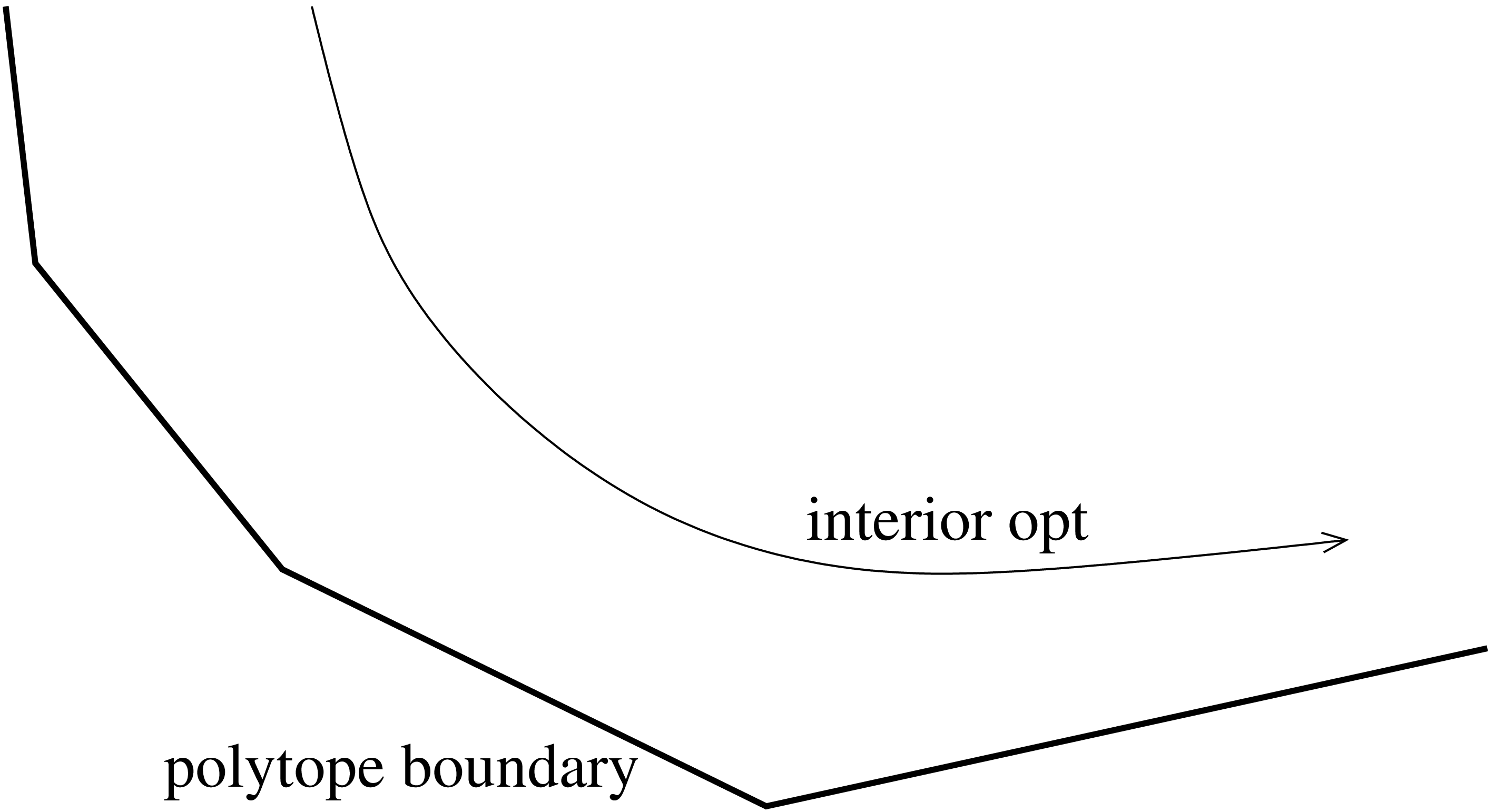
The idea behind interior point algorithms is to avoid turning corners, since this was what led to combinatorial complexity in the Simplex algorithm. They do this by staying in the interior of the polytope, rather than walking along its edges. A given constrained linear optimization problem is transformed into an unconstrained gradient descent problem. To avoid venturing outside of the polytope when descending the gradient, these algorithms use a potential function that is small at the optimal value and huge outside of the feasible region.

To make this idea more concrete, let us consider a specific interior point algorithm due to Ye. Consider the following linear program: \[\begin{aligned} \textrm{minimize\quad} & cx &\\ \textrm{subject to\quad} & Ax &= b\\ & x &\ge 0\\\end{aligned}\] The dual of this program can be written with slack variable \(s\) as follows: \[\begin{aligned} \textrm{maximize\quad} & yb &\\ \textrm{subject to\quad} & yA + s &= c\\ & s &\ge 0\\\end{aligned}\] Ye’s algorithm solves the primal and the dual problem simultaneously; it approaches optimality as the duality gap gets smaller. The algorithm uses the following potential function: \[\phi = A\ln xs - \sum\ln x_i - \sum\ln s_i\] The intent of the \(A\ln xs\) term is to make the optimal solution appealing. Note that \(\ln xs\) approaches \(-\infty\) as the duality gap approaches 0. The two subtracted terms are logarithmic barrier functions, so called because their purpose is to make infeasible points unappealing. When one of the \(x_i\) or \(s_i\) is small, they add a large amount to the potential function. When one of the \(x_i\) or \(s_i\) is negative, these functions are infinitely unappealing. The constant \(A\) needs to be made large enough that the pull towards the optimal solution outweighs the tight constraints at the optimal point.

To minimize \(\phi\), we use a gradient descent. We need to argue that the number of gradient steps is bounded by a polynomial in the size of the input. It turns out that this can be done by arguing that in each step, we get a large improvement. Finally, when we reach a point that is very close to the optimum, we use the trick from last time to move to the closest vertex of the polyhedron.

Conclusion to Linear Programming

Linear programming is an incredibly powerful sledgehammer. Just about any combinatorial problem that can be solved can be solved with linear programming (although many of these special cases of linear programming can be solved more quickly by other methods). For the rest of the lecture, however, we will look at some of the problems that cannot be solved by linear programming.