Structure of Optima in Linear Programs

Lecturers: David Karger
Scribe: Ivaylo Riskov

October 16, 2006

Problem formulation

Consider the linear program \(Ax=b\). We already know that in order to demonstrate a solution or an anti-solution(a certificate for the lack of a solution), we need to exhibit \(x\) in the former case or \(y\), such that \(yA=0\) and \(yb \neq 0\), in the latter case.

Consider the following algorithms to find \(x\):

If \(A\) is square and invertible then \(x=A^{-1}b\)
For general \(A\), we can first find the maximum linear independent subset of columns and if the result is not square, we can discard arbitrary rows to make \(A\) square.

Geometry of Polyhedra

It helps to formalize the notion of a corner.

Theorem: The following three definitions for corner are equivalent:

an extreme point: unique optimum for some objective
vertex: a point which is not a convex combination of two other points in the polyhedron.
basic feasible solution: \(n\) tight linearly independent constraints in dimension \(n\).

Definition: A constraint of the form \(ax \le b\) or \(ax = b\) is tight or active if \(ax = b\).

Definition: For an LP problem in \(n\) dimensions, a point is basic if:

All equality constraints are tight.
\(n\) linearly independent constraints are tight. That is, the point as the intersection of \(n\) independent constraints.

Definition (Basic Feasible Solution): A basic feasible solution is basic and satisfies all constraints.

Lemma: Any standard LP of the form \(\min cx | Ax=b, x \ge 0\) with an optimum (i.e. excluding unbounded or infeasible LP) has one at a basic feasible solution.

Proof. Suppose there exists an optimum \(x\) and it is not a basic feasible solution. Then it satisfies less than \(n\) tight constraints.. This means that there exists a subspace of positive dimension of feasble points that are around \(x\). In particular, there is a line through \(x\) that is feasible in the region near \(x\). If \(d\) is the direction of the line, then \(x \pm \epsilon d\) is feasible for sufficiently small \(\epsilon\).

Consider the objective function \(c(x\pm \epsilon d) = cx \pm c\epsilon d\). \(cd\) must be zero, because otherwsie you could improve on the optimum. Therefore, the optimum is reached anywhere on this line.

If we move along the line, then some \(x_i\) will change. We then pick that direction in which that \(x_i\) increases. We are guaranteed to stop at another constraint. The stopping point is still an optimum, but has at least one more tight constraint.

We can repeat this, until we get \(n\) tight constraints.

In fact, this is an algorithm for transforming any optimum to an optimum at a basic feasible solution. ◻

Note that in canonical form none of the optima might be a basic feasible solution, but any bounded LP has an optimum a basic feasible solution. To illustrate the above consider the example: \(\max y | y \le 2\), \(y = 2\) describes a line that has no corners.

Corollary: All 3 corner characterizations are the same.

Indeed, an extreme point is a basic feasible solution(BFS) since it is a unique optimum for some objective and we know that an optimum is at a BFS. Next, a vertex is a BFS, because if a point is a convex combination of two points, then the line between them is feasible and there are less than \(n\) tight constraints.

This yields the first algorithm for solving LP: try all basic feasible solutions. Given \(m\) constraints and \(n\) dimensions, there are \(m\choose n\) combinations of \(n\) constraints. Those constraints give square constraint matrix \(A'\). We can then invert it to get the candidate \(x={A'}^{-1}b\). The runtime of the algorithm is \(m^{o(n)}\).

Duality

Decision LP

Consider the following decision version of an LP problem:

“Is the optimum less than or equal to \(k\)?” (for minimization problems)

In order to certify that the answer is “yes” we need to exhibit \(x\), such that \(x\) is feasible and \(cx \le k\). But how do we certify “no”?

Goal: Compute a lower bound on \(\min cx | Ax=b, x \ge 0\)

Try to add combinations of existing equations of the form \(a_i x = b_i\). That is multiply \(a_ix\) by some \(y_i\) and add together. \[\sum y_ia_i x = yAx = yb\]

If we can find \(y\) sych that \(yA = c\) then \(yb = yAx = (yA)x = cx\) and this is independent of \(x\) and in particular \(cx\) will stay the same.

We can instead require the looser \(ya \le c\) and then \(yb = yAx = (yA)x \le cx\). (Here we used that \(yA \le cx\) and that \(x\ge0\), so that the inequality is preserved) In other words, \(yb\) is a lower bound on OPT.

Note that the above is true for all \(y\) satisfying \(yA \le c\), so in order to get the best lower bound we are interested in maximizin \(yb\), subject to the constraints \(yA \le c\).

This is a linear program and is the dual of the original LP. It is called the primal LP.

Primal LP: \(\min cx | Ax = b, x \ge 0\)

Dual LP: \(\max by | Ay \le c\)

Weak Duality

Theorem (Weak Duality): If the primal \(P\) is a minimization linear program with optimum \(z\), then it has dual \(D\), which is a maximization problem with optimum \(w\) and \(z \ge w\).

Proof. \(w = yb\) and \(z=cx\) for feasible \(x, z\). Then from \(Ax=b\), \(x \ge 0\), and \(yA \le c\), we get \(w=yb=yAZ\le cx=z\). ◻

Corollary: If \(P\) and \(D\) are both feasible then both are bounded optima.

Converesly, if \(P\) is feasible and unbounded, then \(D\) is infeasible. In fact, there are four possibilities:

1) both are feasible

2) both are infeasible

3) and 4) one is unbounded, the other is infeasible

If \(P\) is unbounded we say that its optimum is \(+\infty\). If it is infeasible, we say that its optimum is \(-\infty\).

We may ask that if the two linear programs are both feasible and bounded then how close the two bounds can get. Strong duality gives the answer to this question.

Strong Duality

Theorem (Strong Duality): If \(P\) or \(D\) is feasible then \(z=w\).

Proof. We’ll do a proof by picture. Let’s start with \(\min \{yb | yA \ge c\}\). Consider the polyhedron formed by the constraints. If we drop a ball inside, it will stop at the optimum (we can consider the vector \(b\) to point in the direction of the gravity).

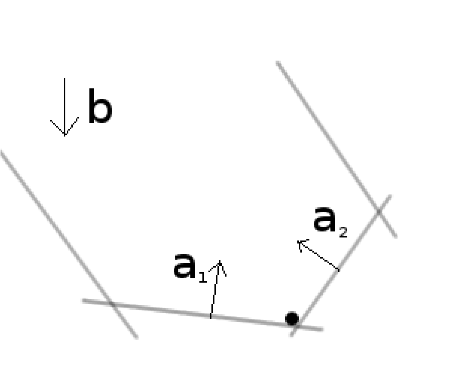
The ball stopped because normal forces exerted by the walls cancel out the force of gravity. Denote the magnitude of the forces with \(x_i\) and the directions in which they point with \(a_i\). Then in order to cancel out gravity, we need: \(\sum a_i x_i = b\). Also note that the forces always push, they don’t pull, so \(x_i \ge 0\). Therefore, \(x\) is feasible in the primal LP.

Note also that only the forces touching the ball can exert force, so if \(y a_i \ge c_i\) then \(x_i = 0\). This is equivalent to saying \((c_i - y a_i) x_i = 0\). Either \(c_i = y a_i\) or \(x_i = 0\).

Finally, we conclude that \(cx = \sum c_i x_i = \sum y a_i x_i = yAx = yb\).

The explanation why \(\sum c_i x_i = \sum y a_i x_i\) is the following: either \(c_i = y a_i\), in which case the terms on the two sides are equal, or \(x_i=0\), in which case both terms, \(y a_i x_i\) and \(c_i x_i\), drop out from their respective sums. ◻